When I started to work for my current company, I have struggled to get one simple overview of this universe. Instead I had to consult many sources, lot of them were going deep into details of one particular financial product. An I was not and still I am not interested in details of investment banking but just needed simple overview.
Over the time I took notes, and kept them for myself, getting information mostly from wikipedia or investopedia. I have posted it here, just in case that it might help someone in the same position that I was.
The world of derivative products is not that complicated. From my (developer's point of view) understanding the basics of derivatives is easy. The finance guys make it bit more complicated by using special vocabulary. For instance selling and option might be called "writing an option". The price of the stock at the time that the broker and the investor exchange the option might be called "Final Reference" or "Spot Price" and so on. You might also understand a product (such as future) but you might get confused by the way it is priced – that is the way that the brokers and investors agree on prices (percentage, basis points, spreads).
Basic vocabulary and terms
There are two entities in this business:
- Asset Manager - a company which has collected large amount of money and invests this money hoping in regular profit. Asset Manager can be also called Buy Side, because historically and probably still he buys more, but he sells as well. So a buy side can be pension fund, mutual fund a big private equity or a hedge fund – in general anyone with enough money.
- Broker - usually a bank. It is the one that gives to Asset Managers what they need. That is the access to the shares and they also create the derivative products that the buy side can use either to risk or to hedge himself while buying some shares. Brokers are called Sell Side as well, because they sell more than buy, even though, they do both (as well as Asset Managers).
Underlying - underlying is anything that you can buy. Usually shares (stocks) or commodities but in some circumstances and underlying can be also a future. The idea is that it “underlies” the derivatives product. For instance you can buy an option on stock of Google. In that case the stock of Google is the underlying. The derivatives are products that are derived from the underlying. An option gives you the right to buy the underlying at some time in the future. A forward will oblige you to buy a stock at the price that you have agreed at some point in the future. A swap will obligate to exchange the underlying for something else. You could create an agreement to swap at some point 200 shares of Google stocks for 1000 liters of beer. This kind of swap would be a derivative with 2 underlyings (shares of google and beer).
Short - means to sell, shorting something means selling that given underlying.
Long - means to buy, being long in something means to buy and underlying and keep it.
List of financial instruments
Financial instruments are anything that you can trade on the markets. Derivatives as such as one category of financial instruments but unlike the basic once, they are "made of" them.
- Equities - stocks, shares
- Debt - bonds or mortages. This products are also called Fixed Income products, because the borrower or issuer aggree on regular payments
- FX - Currencies and Rates
- Commodities - oil, gold, whatever. Not really Financial Instrument, but you can trade it and the derivatives can be based on these as well
- Derivatives - further described in this article. Products derived from all of the other once with additional conditions and rules
Financial Derivatives
This list of financial derivatives is definitely not complete and it is just a try for some logical segregation (which can be sometimes quite hard in this field)
- Options and stratgies - Options give the right to buy or sell and are a basic building block. Two or more options in the same time form strategies, which give interesting exposures.
- Forwards and Futures - the obligation to buy something in the future for fixed price.
- Convertible Bonds - enable the change of a bond into stock
- Swaps Variance, Volatility or Return Swaps - basically exchanging performance or volatility of one stock for other stock's
- ETFs - Exchange-Traded Fund. Can be seen as a stock composed of other stocks
- Others: Autocallables, Accumulators, Program Trading and many other magic stuff
Options
There are two basic types of Options: CALL which gives the owner the right to buy and PUT giving the owner the right to sell. These two basic types can then be composed to form a "strategy". Strategy is just a fancy world used for buying or selling two options at the same time. As you can see later one can choose to do that for multiple reasons.
Call Option
Call is the right, but not the obligation to buy given underlying (stock or commodity) at given price until given date.
A trader who believes that stock's price will increase can buy the right to purchase the stock (he buys call option) at a fixed price, rather than just purchase the stock itself. He would have no obligation to buy the stock, only the right to do so until the expiration date. The price that he will pay for that option is called Premium. If the stock price at expiration (also called Spot Price) is above the agreed price (also called Strike) by more than the premium paid, he will profit i.e. if S>X, the deal is profitable. If the stock price at expiration is lower than the exercise price, he will let the call contract expire worthless, and only lose the amount of the premium. The option is less expensive than the shares itself. For less money the trader can control larger number of shares. That is why we talk about leverage.
Options parameters:
- Premium - the priced paid for the option
- Strike - the agreed price at which the underlying will be bought
- Expiry date (maturity) - the date at which the option expiries (until when you can use it)
- Settlement- either the real underlying is exchanged at expiration date ("Physical") or money is exchanged in place of the underlying ("Cash").
To visualize the options and other derivatives one can use the pay-off charts. On the X-axes of the charts we have the price of the underlying (commodity or stock) and on the Y-axes we have the total profit.

Put option
Put option gives the owner the right to sell the stock for given strike price, otherwise all other parameters are the same.
A trader who believes that a stock's price will decrease can buy the right to sell the stock at Strike price. He will be under no obligation to sell the stock, but has the right to do so until the expiration date. Logically the one who sold him the option will have buy the stock from him (if at some point the option will really get used) If the stock price at expiration is below the exercise price by more than the premium paid, he will profit. If the stock price at expiration is above the exercise price, he will let the put contract expire worthless and only lose the premium paid. Again here are the 2 pay off chats. If you bought a PUT for a MSFT stock with strike 100 for 10 dollars, you bought yourself the right to sell MSFT stock for 100 dollars. Now if the price is 90, you didn't lose anything but did not get anything either. On the other hand if the price did not move and it is still 100, you lost your 10 dollars. That shall be clear from the pay-off chart.

One has to understand, one the market one can buy or sell both types CALLs and PUTs. The outcome of each operation is different. The following chart, shows all 4 operations that can be done.

Delta and Implied Volatility
Delta always and implied volatility sometimes are parameters that the brokers provide with the price of the option, when they want to sell you one.
Delta expresses in percent the change in the price of the option with respect to change in price of the underlying. That is how much will the option price change if the underlying stock moves up or down. Delta is one of the so called Greeks that are briefly discussed later. Delta is expressed in percentage. If a stock costs 10$ and an option (with some maturity) is selled for 5 dollars and the Delta of the option is 50%, then if the stock goes to 11$, the option will go to 5.5%. That is called a delta adjustment. The broker at some point proposes a price to the investor and provides the delta as well. If the investor buys in next hour, he knows what the price of the option will be at the deal time.
Delta is always positive for a CALL and negative for a PUT. If a price of the underlying goes down, then the price you pay for the right to sell such share on some fixed price goes up. If the price of the underlying falls from 10 to 1, and you had an option giving you the right to sell for 5, you are lucky since, since you will be selling much above the market. It's clear that price of such option goes up. The reverse is true for the call. If the price of the underlying goes from 10 to 15, and you wanted to buy an option with strike 12. The broker was willing to sell you such option for 11 before, but it's price went definitely up.
Implied Volatility is another parameter sometimes provided by the brokers when giving the prices. In order to provide the price for any given option, the broker estimates the volatility of the market in the future. Implied Volatility is such estimation. Options are priced by using different variations of Black Sholes furmula. The basic idea behind this formula states, that the price of an option does depend only on it's parameters, current price of the option and the estimated volatility of the market. Of course when a broker gives a price of an option, the price will depend also on other factors, such as whether the broker has any shares of the given underlying already. But in theory, the broker could just provide the estimated volatility that he puts into his model and that is enought to calculate the price.
Options trading and hedging against delta adjustment
When a trader wants to obtain an option, he will specify the parameters and ask brokers whether they can give him such contract. The broker will give to the trader the price for such contract and also the delta. That is the rate at which the contract price will change with respect to the change in the underlying.
If the contract is big enough, the broker might need some time to acquire enough shares. Also the buyer might take some time to decide whether to buy or not. So after all this delay, the price of the option contract has changed by delta*(underlying price change). The buyer might have lost money.
To evict such situation, options hedging is used. In this situation, the broker will buy from the buyer of the option such amount of shares of the given underlying, so the change of the price of the option contract will be completely mitigated by this operation.
Strategies based on options
Calls and Puts can be bought or selled in the same time with diferent parameters. This results in diferent pay-offs of such operations. Buying or selling multiple options at the same time in the same contract is called buying a "Strategy". Here is probably non-complete list of strategies:
Call spread
This strategy consists of two calls with the same expiry. The first one with smaller strike is sold and other with higher strike is bought.
The payoff is shown bellow. Call spread behaves liked to underlying, but the maximum profit and maximum loss values are limited by the strike prices of the calls.
Analogically to call spread, put spread is a strategy composed of two put options, with the same expiries and different strikes.
Strangle
Strangle allows the holder to profit based on how much the price of the underlying security moves, with relatively minimal exposure to the direction of price movement. Long stangle is composed of long call and long put, with same expiries. The profit potential is unlimited, the strategy may be used in volatile markets.
Short strangle is composed of short put and short call with same expiries and it is profitable if the price of the underlying does not move much and the profit is limitted to the premiums obtained, otherwise the potential loss is unlimited.

Straddle
Very similar to strangle, Long Straddle is a long call with a long put, with same strikes and expiries.
Strategy involving the purchase or sale of particular option derivatives that allows the holder to profit based on how much the price of the underlying security moves, regardless of the direction of price movement. Long straddle = long call option + long put option – same strike and expiry. As for strangle, this strategy might be usefull in highly volatile markets.
Again Short straddle is like short strangle, but strike is the same. The price has to stay very close to the strike for a profit based on premiums.

Butterfly
Limited risk, non-directional options strategy that is designed to have a large probability of earning a limited profit when the future volatility of the underlying asset is expected to be lower than the implied volatility.

Risk reversal
Selling an out of money put and buy out of money call with same maturity. An investor wants to go long in the underlying but instead of going long on the stock, he will buy an out of the money call option, and simultaneously sell an out of the money put option. Presumably he will use the money from the sale of the put option to purchase the call option. Then as the stock goes up in price, the call option will be worth more, and the put option will be worth less. If an investor holds the underlying and sells a risk reversal, then he has a collar position.
The pay-off is exactly the same us holding the underlying stock. One could use risk reversal to speculate on a stock without holding the stock.

Collar
- Long the underlying
- Long a put option at strike price X (called the "floor")
- Short a call option at strike price (X+a) (called the "cap")
Latter two are a short Risk reversal position,so we can say Underlying - Risk reversal = Collar. The profit or loss on underlying are very limited.
The premium income from selling the call reduces the cost of purchasing the put.

Condor
Stragy with limited risk, non-directional (the same result if underlying moves either way) with limited profit when the underlying security is perceived to have little volatility.
- Sell 1 In The Money Call
- Buy 1 In The Money Call (Lower Strike)
- Sell 1 Out of The Money CALL
- Buy 1 Out of The Money CALL (Higher Strike)
Maximum profit for the long condor option strategy is achieved when the stock price falls between the 2 middle strikes at expiration. It can be derived that the maximum profit is equal to the difference in strike prices of the 2 lower striking calls less the initial debit taken to enter the trade.

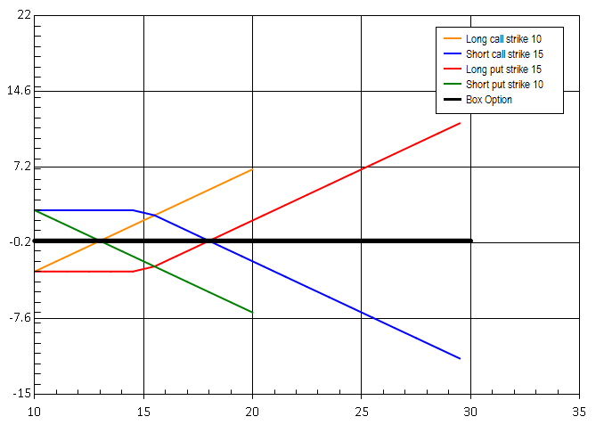
Box option
Combination of 4 basic legs, that achieves neutral interest rate position - riskless payoff.
- Long call strike 10
- Short call strike 15
- Long put strike 15
- Short put strike 10
The strategy has constant payoff, in ideal case the net premium paid for the strategy should be equal to the payoff. However the comission will reduce the profitability to nothing. Might be seen as a form of lending money on markets.
Barrier options
TODO!!!
Warrants
Warrants have the same parameters and behave just like options. There are few differences:
- They are not publicly traded, not listed, like OTC options.
- The expiration period is usually in years.
- Once the warrant is exercised the new outstanding shares of company are created. In case of options, no new shares are issued, the writer of the option has to buy them on the market.
- Often used as alternative to employees stock options.
Specifying option and it's price
This part is not about the actual pricing of options, that is determining the price. This is more about how options are exchanged on the market, in what units the prices as exchanged.
- Fixed price per contract
- In percentage
- Spread between legs
- Pricing by strike
- Total premium for multilegs
Forwards & Futures
By buying a forward or future, you have the right but also the obligation to buy given underlying at the selected price. Both are part of Delta One products. Since the price of the future moves the same way as the price of the underlying. Futeres unlikely to forwards are listed, standardized contracts. That means they can be bought on an exchange. Forwards are pure OTC products - not standardized at all.
Futures or Forwards have the same parameters as options, though in the majority of cases, no strike is specified. That is because the price at which the underlying will be exchanged at the expiration date, is defined solely by the market. Typically futures prices are listed on the market. For instance the current price of SPX Indice might be 2000 and the future which expires next month might be at 2050.
Pricing of futures
Futures are delta-one derivatives. The price of the future changes hand in hand with the price of the underlying (if the stock goes up one dolar, the future on the same stock in 3 months will go up as well by one dollar). That affects the way that futures are priced. Since typically the future price is always specicied with respect to the current stock price, there are 2 common ways of pricing futures:
TODO!!!
- Net Basis - the difference between stock price and future price is given by the broker in basis points.
- In Percentage - the future price is given as the percentage of current price. For bullish stock that will be greater than 100% and for bearish stocks that will be lower than 100%.
Future and Forward Rolls
Rolls enable the holder of given future to keep the position in the underlying when his future is about to expire.
Convertible Bonds, Reverse Convertible Bonds
These two derivatives at some point allow or force the holder to convert bonds into shares.
Convertible Bonds
Convertible Bond is a contract which allows the conversion of listed corporate bonds into the underlying equity. This is available only on listed companies that issue as well bonds to finance their operations. Converts are listed on exchanges. The companies issue the CBs just like the bonds the are underlying the converts.
From certain point of view, CB can be seen as an option, because if underlying stock behaves achieves certain performance, the owner will become the proprietary of the stock, if not, he will keep the bonds with regular return. For that reason, it makes sense to provide Delta while pricing Convertible Bonds, since the price of the CB will move with respect to the underlying share.
Convertible bond thus has the power of option and can be leveraged to obtain the underlying equity. It will be however more expensive than CALL option becase one pays for the bond as well.
Reverse Convertibles
Holder of a Reverse convertible is regulary paid a coupon as if he would be holding a standard bond. On the upside if the shares of the underlying company (and that can be any company, not just the issuer of the original bonds) fall bellow certain PUT like Strike. His bonds will convert into the stocks of this company
Swaps
Swaps as the name suggest are contracts that specify an exchange between the buyer and the seller of the contract. There are various types, depending on what is exchanged: Commodity, Interest Rate, Volatility or Variance.
Variance and Volatility Swaps
Volatility measures the magnitude of movements for given stock. Standard deviation is used to express the volatility of the stock. Variance is the square of standard deviation, so in a sense just amplified volatility.
Volatility or Variance swap allow the investor to bet on the volatility. The investor specifies a volatility level which he expects (striked volatility) and if the volatility goes over this level, he gets paid a bigger payoff. The payoff is specified as:
PayOff = VegaAmount (RealVolatility – Volatility Striked)/ RealVolatility
The bigger the difference between the Real Volatility and the Striked volatility is, more money does the buyer of such swap gets. The whole amount is multiplied by a multiplier called "Vega Amount". Vega is on of the greeks which meassures the sensitivity of an option to the change in the volatility of the option. There is however no connection here. It's just the term used on the markets for this multiplier.
Total Return Swaps
TRS allows the buyer to exchange the performance of certain stock for the performance of standard interest rate. The buyer can for instance bet on the performance of certain underlying (eg. MSFT stock) against a standard interest rate for standard period. For instance Euribor 6M is the interest rate provided by ECB (European Central Bank) for next 6M. That might be 2% fo example. The buyer believes that MSFT will beat that and asks the seller to pay him the difference if that is the case. The seller, for certain comission will do that. That allows the asset manager to bet on performance without owning the underlying shares.
ETFs
Exchange Traded Funds are compositions of stocks, that usually track an index or a sector. They are listed and traded like regular stocks. They companies that emit ETFs thus enable the asset managers to invest into whole sectors or regions, without the need of knowing the details of the markets.
Net Asset Value
Common to all funds which invest into stocks. At the end of the day the NAV of the fund is calculated as the sum of all the stocks own by the fund, divided by the number of shares.
ETFs however are listed themselves and traded on the market so beside the NAV they also have the market value. Their market value can be bellow or over the NAV.
Settlement date
The date when you need to the money to buy your ETF or when you will receive the money for selling. For ETFs it is 3 days after the deal (for some traditional reasons, I suppose).
Creation Redemption
Creation is the process of emission of ETF shares. ETF is supposed to track a sector or index and has exact composition. The company issuing ETFs needs to aquire the stocks that form the ETF to emit it. Since one share of ETF has exact composition, the issuer needs to aquire that exact amount to be able to sell that one share of ETF with certain comission.
Redemption is the reverse process. The issuer will buy the ETFs from the owners and give them back the underlying shares, or equal amount in cash.
This process is essential and allows the ETF to always trade around it's NAV. If the demand fo some ETFs (eg. ETF mirroring Asian construction market) would be too high, the prices would go up too much and get too far away from the real prices of the shares of the mirrored companies. The issuer can in that case emit more shares of the ETF. On the other hand if investors start to sell certain ETF too much and don't believe in the sector, the redemption process can reduce the quantity of the ETFs and stabilize the price which would go down too much otherwise.
Other crazy stuff
Autocallables
TODO!!!
Program Trading
An asset manager might interested in investing in sectors or countries, not exact shares. ETFs are one way to get there, Program Trading might be the other way. PT are basket trades (buying multiple underlyings in same time) and are very big in size, the buyer specifies the total amount of the traded volume (total notional) and might provide also the number of stock he wants to buy in the future. Then he gives multiple characteristics such as the percentage per country or sector. For instance 10% in US, 30% in UK and 25% in Telecom, 50% in services and so own. He also asks certain parameters such as how much this composition should track some index. This is done usually by setting the Beta in percent versus some index like SPX. The seller of such contract than provides price and some (huge) commission.
The investor will do such a trade when he wants to invest big amount of money in the same time to multiple markets. Usually the trade composition is determined by dedicated software, hence "Program Trading".